Markov Chains Visualization

This website is created for the purpose of visualizing Markov Chains.

Developed by: Miguel Robles, Kovie Niño, and Zach Noche

Before we get started, look into how Markov Chain works. If you wish to skip, you may collapse the division by clicking the title below.

Want a more detailed explanation? You may find a more detailed explanation of Markov Chains, complete with the Python code used to derive the simulation results shown below, by clicking here:

Datalore Jupyter Notebook

(Note that you need a Jetbrains account to access the link)

A Markov Chain is a random process that undergoes transitions from one state to another on a state space. The defining characteristic is that the probability of transitioning to any particular state depends solely on the current state and time elapsed, and not on the sequence of states that preceded it.

Memorylessness

Memorylessness is a key feature of Markov Chains. If we look at the example, previous states do not matter as the next state solely relies on the probabilities from the current state.

Stochastic Process

A stochastic process is a collection of random variables: \{X_t,t \in I \}, Where X_t is the set of random variables at time t, and I is the index set of the process.

Markov Chain is a type of Stochastic Process

Markov Process

A sequence of random states S1, S2, ..., with the Markov property, is called a Markov chain. This process can be entirely defined by the state space and transition matrix.

State Space: A set of all possible states
Transition Matrix: A matrix wherein each entry on the i-th row and j-th column (aij) represents the probability of moving from state i to state j.

Let's create a simple markov chain.

Markov Transition Graph from Deparkes

	Sunny	Rainy	Cloudy
Sunny	0.7	0.2	0.1
Rainy	0.1	0.6	0.3
Cloudy	0.2	0.5	0.3

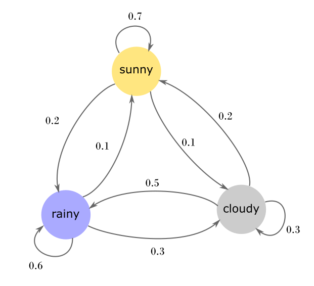
The state space represents the weather conditions. The transition matrix weather chain represents the probabilities of moving from one weather condition to the other. This matrix is in column form and each column represents the probabilities of going from one state to another.

Example:

The 'Sunny' list [0.7, 0.1, 0.2] indicates the probabilities of the following transitions:

Transitioning from 'Sunny' to 'Sunny': 0.7
Transitioning from 'Rainy' to 'Sunny': 0.1
Transitioning from 'Cloudy' to 'Sunny': 0.2

The 'Rainy' list [0.2, 0.6, 0.5] indicates the probabilities of the following transitions:

Transitioning from 'Sunny' to 'Rainy': 0.2
Transitioning from 'Rainy' to 'Rainy': 0.6
Transitioning from 'Cloudy' to 'Rainy': 0.5

The 'Cloudy' list [0.1, 0.3, 0.3] indicates the probabilities of the following transitions:

Transitioning from 'Sunny' to 'Cloudy': 0.1
Transitioning from 'Rainy' to 'Cloudy': 0.3
Transitioning from 'Cloudy' to 'Cloudy': 0.3

Initial State Probability

The initial state probability is typically denoted as a vector, where each entry corresponds to the probability of the system being in a particular state at the start. The sum of all probabilities in this vector must equal 1, reflecting the certainty that the system must be in one of the possible states at the beginning.

For example, if we have a Markov chain with states 'Sunny', 'Rainy', and 'Cloudy', we might have an initial state probability vector like [0.5, 0.3, 0.2]. This would mean that at the start, the system has a 50% chance of being in the 'Sunny' state, a 30% chance of being in the 'Rainy' state, and a 20% chance of being in the 'Cloudy' state.

When defining Markov Chains, one can either set an initial state or initial state probabilities. Selecting a sure initial state is simply setting the vector to [1.0, 0.0, 0.0]. In this example this is exactly what we do, making the start state always sunny.

Example Runs from the current set rules:
[Initial: Sunny → Sunny → Cloudy → Rainy → Cloudy → Rainy → Rainy → Rainy → Cloudy → Cloudy → Sunny → End]
[Initial: Sunny → Sunny → Cloudy → Cloudy → Cloudy → Sunny → Sunny → Rainy → Rainy → Rainy → Rainy → End]
[Initial: Sunny → Sunny → Sunny → Sunny → Sunny → Sunny → Sunny → Sunny → Sunny → Sunny → Sunny → End]

N-Step Transition Matrix

What N-Step transition matrix gives us is the probability of reaching a certain future state given the current state at n steps.

A N-Step transition matrix is found by taking the nth power of the original transition matrix. This is based on the principle that the probability of transitioning from one state to another in n steps is the sum of the probabilities of all paths from the initial state to the final state that consist of exactly n steps.

If we want to find the 2-step transition matrix, we compute P^2 (i.e., the matrix product of P with itself). This gives us the probabilities of transitioning from each state to each other state in 2 steps.

One important point to remember is that the process of taking powers of the transition matrix assumes that the Markov chain is time-homogeneous, meaning that the transition probabilities do not change over time.

Get the 2-step transition matrix

	0	1	2
0	0.53	0.31	0.16
1	0.19	0.35	0.28
2	0.25	0.49	0.26

It is telling us here that after 2 steps these are the chances to end up in a certain weather

3 Step and Beyond

After the two step matrix it gets a little tricky as we need to get three and beyond we need to get dot product of the previous step and the current transition which can get tedious as more steps are added. (P^3 = P^2 * P)

	0	1	2
0	0.434	0.372	0.1939
1	0.242	0.496	0.2619
2	0.2759	0.474	0.2499

Steady State

The steady state in a Markov chain is a state where the system's probabilities remain unchanged even after transitions. That is, the system has reached an equilibrium where the distribution of states in the future does not depend on the current state.

The concept of steady state is central to stationary or time-homogeneous Markov chains, where the transition probabilities don't change over time.

1-Step Transition Matrix

	0	1	2
0	0.7	0.2	0.1
1	0.1	0.6	0.3
2	0.2	0.5	0.3

50-Step Transition Matrix

	0	1	2
0	0.3095	0.4523	0.2380
1	0.3095	0.4523	0.2380
2	0.3095	0.4523	0.2380

100-Step Transition Matrix

	0	1	2
0	0.3095	0.4523	0.2380
1	0.3095	0.4523	0.2380
2	0.3095	0.4523	0.2380

What is this all for?

From the result of the steady state we can say the long term probability of the day being a certain weather is dependent on our achieved steady state.

Example

From the results of the weather chain, we can say that the probability of it being sunny is around 31%, rainy 45%, and cloudy 24%.

In a perfect world, where there are no changes due to factors like global warming, and assuming our matrix is correct, if one gathers enough weather data, then we'd expect these rough proportions.

Let's try the diagram below!

You can try to create your own Markov Chain and see how it works.

Markov Chain Diagram

Note: The diagram is interactable, you can drag the nodes around and zoom in and out.